Spice up your C++ web app with visualizations
By Stefan Verhoeven, Faruk Diblen, Jurriaan H. Spaaks, Christiaan Meijer, and Adam Belloum.
In a previous blog we found the root of an equation using the Newton-Raphson algorithm implemented in C++ and compiled to a WebAsssembly module. In this blog, we’re going to expand on that by visualizing the iterations that Newton-Raphson used to get from the initial guess to the estimate of the root.

Iterations
The Newton-Raphson algorithm approximates the value of the target equation’s root in a series of iterations. We capture the data of each iteration using the following struct:
x: x value, starting with the value ofinitial_guessand ending with the estimate of theequation's rooty: result of passingxthroughequationslope: result of passingxthroughderivative
Extending the NewtonRaphson class accordingly yields the following header file:
The do loop in newtonraphson.cpp is updated to include a push_back to the iterations vector. This way, we can record the value of relevant variables in each cycle, as follows:
Before we go into the Emscripten world, let’s first test our C++ code. We can check if the iteration property is populated correctly, by extending the command line interface we made in the previous blog as follows:
Compile it with:
g++ -o cli.exe problem.cpp newtonraphson.cpp cli.cppRun with:
./cli.exe
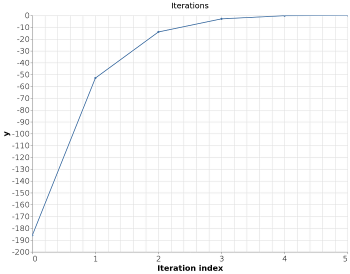
index = 0 x = -4.00 y = -186.00 slope = 128.00 delta_x = -1.45
index = 1 x = -2.55 y = -52.99 slope = 59.29 delta_x = -0.89
index = 2 x = -1.65 y = -13.97 slope = 29.63 delta_x = -0.47
index = 3 x = -1.18 y = -2.89 slope = 17.83 delta_x = -0.16
index = 4 x = -1.02 y = -0.28 slope = 14.40 delta_x = -0.02
index = 5 x = -1.00 y = -0.00 slope = 14.01 delta_x = -0.00
The last iteration has x = -1.00, which is what we expected.
Bindings
Emscripten can handle simple types like float and int, but needs help exposing more complex types to JavaScript like the iterations property. We need to usevalue_object to expose the Iteration struct and register_vector as the iterations property type.
So the bindings look like this:
We can now compile our C++ code to a WebAssembly module with Emscripten using emcc command, exactly like we did before:
emcc -I. -o newtonraphson.js -Oz -s MODULARIZE=1 \
  -s EXPORT_NAME=createModule --bind \
  problem.cpp newtonraphson.cpp bindings.cpp
To get the iteration data in JavaScript we use the following code
Let’s have a look at the data we want to plot, by logging it to the console with console.log(JSON.stringify(iterations, null, 2)), which should return the following data:
Great, that looks very similar to the output we got from the command line.
Vega-Lite specification
There many ways to do visualizations on the web. One of our favorites is Vega-Lite, a JavaScript library which describes a plot using a JSON document called a specification.
The root finding algorithm tries to find the x where y is zero using a series of iterations. Let's plot the iteration index against the y found in each iteration to see how quickly it converged to an answer.
The generic structure of our Vega-Lite specification looks like this:
To render a specification we need to use the vegaEmbed(element, spec) method which accepts an HTML element and a Vega-Lite specification.
Combining the three snippets above (get iteration data, Vega specification and vegaEmbed) and filling in their respective details yields an HTML document with the complete web app:
We’ll need a web server to display the HTML page in a web browser. For this, we’ll use the http.server module from Python 3 again to host all files on port 8000, like so:
python3 -m http.server 8000When we visit the web page at http://localhost:8000/scatter.html, we will be greeted by the following plot. We can zoom with the mouse wheel and pan by dragging. Hovering over a point shows a tooltip with relevant data at that point.

Advanced plot
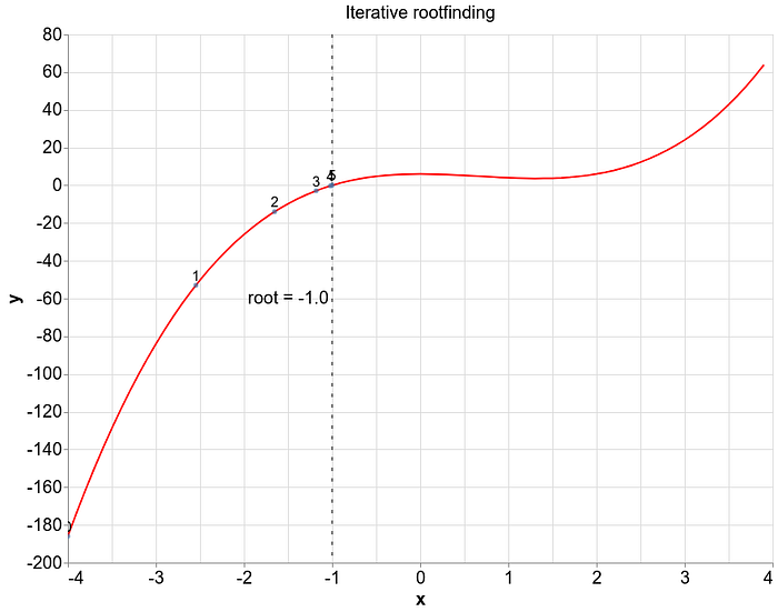
In the first blog of this series we plotted the equation and root as
It would be nice to write a specification of this plot together with the iterations that the root finding algorithm went through. Vega-Lite can superimpose one chart on top of another with the keyword. Let’s construct each layer separately and then superimpose them at the end.
The 2x³ — 4x² + 6 equation is plotted by using a sequence generator to generate a range of x values and a formula transform is used to calculate the y values.
To show where the root is, we draw a dotted vertical line using a rule marker at x = -1 and label it root with a text marker.
When we plot the x and y of each iteration we can no longer see the order of iterations, so we will use a text marker above each circle to indicate which iteration it belongs to.
Superimpose the equation line, root ruler, and iteration scatter into a single visualization with:
The HTML page with all JavaScript put together to make a composite plot is available here.
Visiting the page should give us a plot like

Wrap up
In this blog we have learned how to get complex data types from a WebAssembly module using Emscripten bindings and how to write a Vega-Lite specifications to get interactive visualizations.
Other blogs of the series that might be of interest
We’ll wrap up the series in a final blog that combines the topics of the whole series in a full-featured web application.
This blog was written by the Generalization Team of the Netherlands eScience Center. The team consists of Stefan Verhoeven, Faruk Diblen, Jurriaan H. Spaaks, Adam Belloum and Christiaan Meijer. Feel free to get in touch with the generalization team at generalization@esciencecenter.nl.
If you enjoyed this article, leave a comment and give us a clap!
These blogs were written as part of the “Passing XSAMS” project. To learn more about the project, check out its project page.
