Speed up your Python code using Julia
Part two of the series on achieving high performance with high-level code
By Abel Soares Siqueira and Faruk Diblen

In part 1 of this series, we set up an environment so that we can run Julia code in Python. You can also check our Docker image with the complete environment if you want to follow along. We also have a GitHub repository with the complete code if you want to see the result.
Background
On the blog post, 50 times faster data loading for Pandas: no problem, our colleague and Senior Research Software Engineer, Patrick Bos, discoursed about improving the speed of reading non-tabular data into a DataFrame in Python. Since the data is not tabular, one must read, split, and stack the data. All of that can be done with pandas in a few lines of code. However, since the data files are large, performance issues with Python and Pandas now become visible and prohibitive. So, instead of doing all those operations with pandas, Patrick shows a nice way of doing it with C++ and Python bindings. Well done, Patrick!
In this blog post, we will look into improving the Python code in a similar fashion. However, instead of moving to C++, a low-level language considerably harder to learn than Python, we will move the heavy lifting to Julia and compare the results.
A very short summary of Patrick’s blog post
Before anything, we recommend checking Patrick’s blog post to read more into the problem, the data, and the approach of using Python with C++. The short version is that we have a file where each row is an integer, followed by the character #, followed by an unknown number of comma-separated values, which we call elements. Each row can have a different number of elements, and that’s why we say the data is non-tabular, or irregular. An example file is below:
From now on, we refer to the initial approach of solving the problem with Python and pandas as the Pure Python strategy, and we will call the strategy of solving the problem with Python and C++ as the C++ strategy.
We will compare the strategies using a dataset we generated. The dataset has 180 files, generated randomly, varying the number of rows, the maximum number of elements per row, and the distribution of the number of elements per row.
Adding some Julia spice to Python
The version below is the first approach to solve our problem using Julia. There are shorter alternatives, but this one is sufficiently descriptive. We start with a very basic approach so it is easier to digest.
You can test this function on Julia directly to see that it works independently of Python. After doing that, we want to call it from Python. As you should know by now, that is fairly easy to do, especially if you use the Docker image we have created for Post 1.
The next code snippet includes the file that we created above into Julia’s Main namespace and defines two functions in Python. The first, load_external , is used to read the arrays that were parsed by either C++ or Julia. The second Python function, read_arrays_julia_basic , is just a wrapper around the Julia function definition in the included file.
Now we will benchmark this strategy, which we will call the Basic Julia strategy, against the Pure Python and C++ strategies. We are using Python 3.10.1 and Julia 1.6.5. We run each strategy three times and take the average time. Our hardware is a Notebook Dell Precision 5530, with 16 GB of RAM and an i7–8850H CPU, and we are using a docker image based on Ubuntu Linux 21.10 to run the tests (from inside another Linux machine). You can reproduce the results by pulling the abelsiqueira/faster-python-with-julia-blogpost Docker image, downloading the dataset, and running the following command in your terminal:
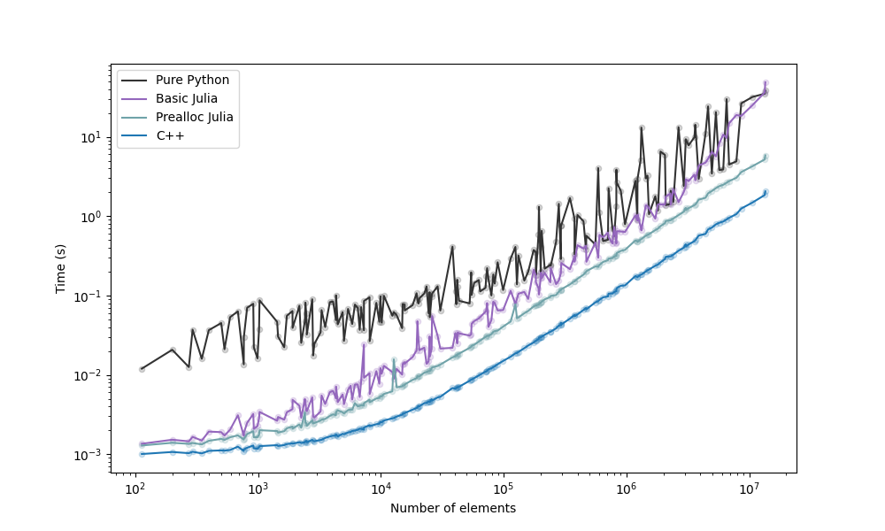
$ docker run --rm --volume "$PWD/dataset:/app/dataset" --volume "$PWD/out:/app/out" abelsiqueira/faster-python-with-julia-post2See the figure below for the results.


A few interesting things happen in the image. First, both Pure Python and Basic Julia have a lot of variability with respect to the number of elements. We believe this happens because the code’s performance is dependent on the number of rows, as well as the structure distribution of elements per row. The code allocates a new array for each row, so even if the number of elements is small, if the number of rows is large, then the execution will be slow. Remember that our dataset has a lot of variability on the number of rows, maximum elements per row, and distribution of elements per row. This means that some files are close in the number of elements but may be vastly different. Second, Basic Julia and Pure Python have different efficiency profiles. Our Julia code must move all stored elements into a new array for each new row that it reads, meaning it allocates a new array for every row.
The code for Basic Julia is simple and does what is expected, but it does not pre-allocate the memory that will be used, so that really hurts its performance. In low-level languages, that would be one of the first things we would have to worry about. Indeed, if we look into the C++ code, we can see that it starts by figuring out the size of the output vector and allocating them. We need to improve our Julia code at least a little bit.
Basic improvements for the Julia Code
The first version of our Julia code is inefficient in a few ways, as explained above. With that in mind, our first change is to compute the number of elements a priori and allocate our output vectors. Here is our improved Julia code:
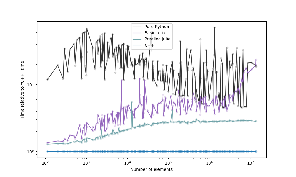
Here, we use a dictionary generator comprehension, which has the closest resemblance to the data. This allows us to count the number of elements and keep the values to be stored later. We also use the package Parsers, which provides a slightly faster parser for integers. Here is the updated figure comparing the three previous strategies and the new Prealloc Julia strategy that we just created:


Now we have made a nice improvement. The results more consistently depend on the number of elements, like the C++ strategy. We can also see a stabilization of the trend that Prealloc Julia follows. It appears to be the same as C++, which is expected since the performance should be linearly dependent on the number of elements. For files with more than 1 million elements, the Prealloc Julia strategy has a 5.83 speedup over the Pure Python strategy, on average, while C++ has a 16.37 speedup, on average.
Next steps
We have achieved an amazing result today. Using only high-level languages, we were able to achieve some speedup in relation to the Pure Python strategy. We remark that we have not optimized the Python or the C++ strategies, simply using what was already available from Patrick’s blog post. Let us know in the comments you have optimized versions of these codes to share with the community.
In the next post, we will optimize our Julia code even further. It is said that Julia’s speed sometimes rivals low-level code. Can we achieve that for our code? Let us know what you think and stay tuned for more!
Many thanks to our proofreaders and reviewers, Elena Ranguelova, Jason Maassen, Jurrian Spaaks, Patrick Bos, Rob van Nieuwpoort, and Stefan Verhoeven.

