Breaking the barrier: fluid simulations parallel-in-time.
These days computers are growing faster only by adding more cores and increasing parallelism of the programs. As an example, suppose we are computing the turbulent flow around an airfoil. This is a problem that is very intensive to compute so we’d want to parallelise it.
Parallel-in-space, and scaling of overhead
The traditional approach is to divide the volume of our simulation into different domains, and give each domain to a different processor. After each time-step the changes in each domain need to be communicated between the processors. This adds overhead to the computation. Each time we split the volumes in half we can potentially double the speed in which we get our answer, but this is mitigated by the fact that we also increase the amount of communication needed between the compute nodes.
This principle of balancing processing power versus communication overhead is a universal one. There always seems to be a barrier to how many processors we can use for solving a problem. The question is then, how can we break this barrier, how can we parallelise our computation even further? This is the point where we go parallel-in-time.
Parallel-in-time, but how?
At first the notion of parallel-in-time integration often is counter intuitive. The problem of simulation a fluid (and many other computations like it) is inherently sequential. The change in a state of a physical system always depends on the current state of the system. How then, do we compute the future in parallel with the past?
Parareal
A simple method that, in theory, gives decent speed-ups is Parareal. It was invented in 2001 by Lions, Maday & Turinici. The introduction of Parareal was largely what got the current surge in parallel-in-time methods started, since it is the first algorithm that showed enough promise to give a real speed up. Also, it is relatively simple to explain.
Coarse & Fine
Parareal works by defining a coarse and a fine algorithm. The coarse algorithm should be cheap to compute, possibly a low order integration, on a coarse grid, possibly also with reduced model complexity and with a large time-step. The fine integrator on the other hand, is the expensive algorithm often computed on a finer grid, with all necessary physics included.
The first step of Parareal is to get an initial guess for the evolution of the system by taking the result of just the coarse integrator. We use this initial guess to start the fine integrator at each time-step simultaneously. Since we already have an initial guess for each time-step (on the coarse grid), we can perform the fine integration in parallel.
At the end of this step each of the fine integrators will be slightly off, because they started from a wrong first estimate. We can try to correct the results of the fine integrators. Several iterations of fine integration followed by correction will be needed.
The quality of the Parareal algorithm depends heavily on the accuracy of the coarse integrator.
We only get a speed-up if the algorithm converges in fewer iterations than our number of time-steps. Also note that while we get our answer faster, we need to do a lot more work to get it.
The Bay of Fundy
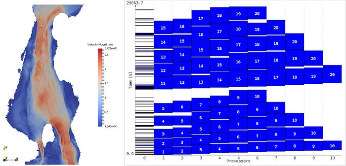
An example of a successful application of Parareal in hydrodynamics was presented by Eghbal, Gerber & Aubanel (2016) [doi:10.1016/j.jocs.2016.12.006]. They implemented Parareal on top of an existing (proprietary, sad enough) GPU hydro code with the aim of modelling hydro turbine tidal power generation in the Bay of Fundy.

The Gantt chart on the right shows the work being done by 10 processors. Eghbal et al. divided the work in multiple time ‘windows’, two of which are shown here. In each window we see that Parareal converged in 5 iterations. To save data transfer in the correction step, each processor works on successive time-steps. This way only the data of the coarse integrator has to be propagated between processors.
Difficulties
One area where Parareal is reported to go wrong is with oscillating systems. The coarse integrator usually gives a result that is out-of-phase with the real solution. Attempts have been made to do phase-correction on top of Parareal, but this is still very much a topic of research.
Beyond Parareal
There are many more methods for parallel-in-time integration. One example is Multigrid Reduction in Time or MGRIT. MGRIT can be seen as a generalisation of Parareal. It has more flexibility in the ways to correct the results from the fine integrator, and can be used in conjunction with multi-grid method in space. An implementation of MGRIT is available in the XBraid package.
Fair warning
There are reports of significant speed-ups with parallel-in-time methods but this comes with a warning. There is a big investment into tuning the system. A lot of work goes into making current parallel-in-time methods perform faster than sequential methods. In the case of Parareal, this means finding a good model for the coarse integration.
Stay green
To recap, our question was: How do we compute past and future in parallel? The answer: by wasting a lot of computational power. In these days of ecological responsibility and green computing, wasting valuable processor cycles seems like a bad idea. Even if you succeed in getting a speed-up, you still need to convince your local super computing facility why you need all this.
We may find however, that in some cases there is no other way forward. As the number of cores on a machine keep increasing, we need to be more creative in utilizing the computational power we’re given.
Further reading
The field of parallel-in-time methods is still young. At http://www.parallel-in-time.org there is a collection of scientific papers and computer codes. A good review on available methods is “50 years of parallel-in-time” by Martin Gander.

